Working with the dashboard

The dashboard shows you all sub-components of biopb, and allows you to:

• observe your agent: lets you watch what the agent runs, step in when something goes wrong, and save the whole session as a notebook for the record.
• change biopb settings: edit/rewrite the config file of biopb or restart the data server with a new configuration
• view data: see your microscopy data via a web interface without connecting to an agent or start napari

Opening it

Open biopb dashboard like any other app on your desktop, or, if you are a terminal user, run biopb dashboard in your terminal

What's on it

Four panels, each covering one piece of the system.

The dashboard: the data plane and its controls, the algorithm servers your agent can reach, which agents biopb is registered with, and every live session with a link to watch it.

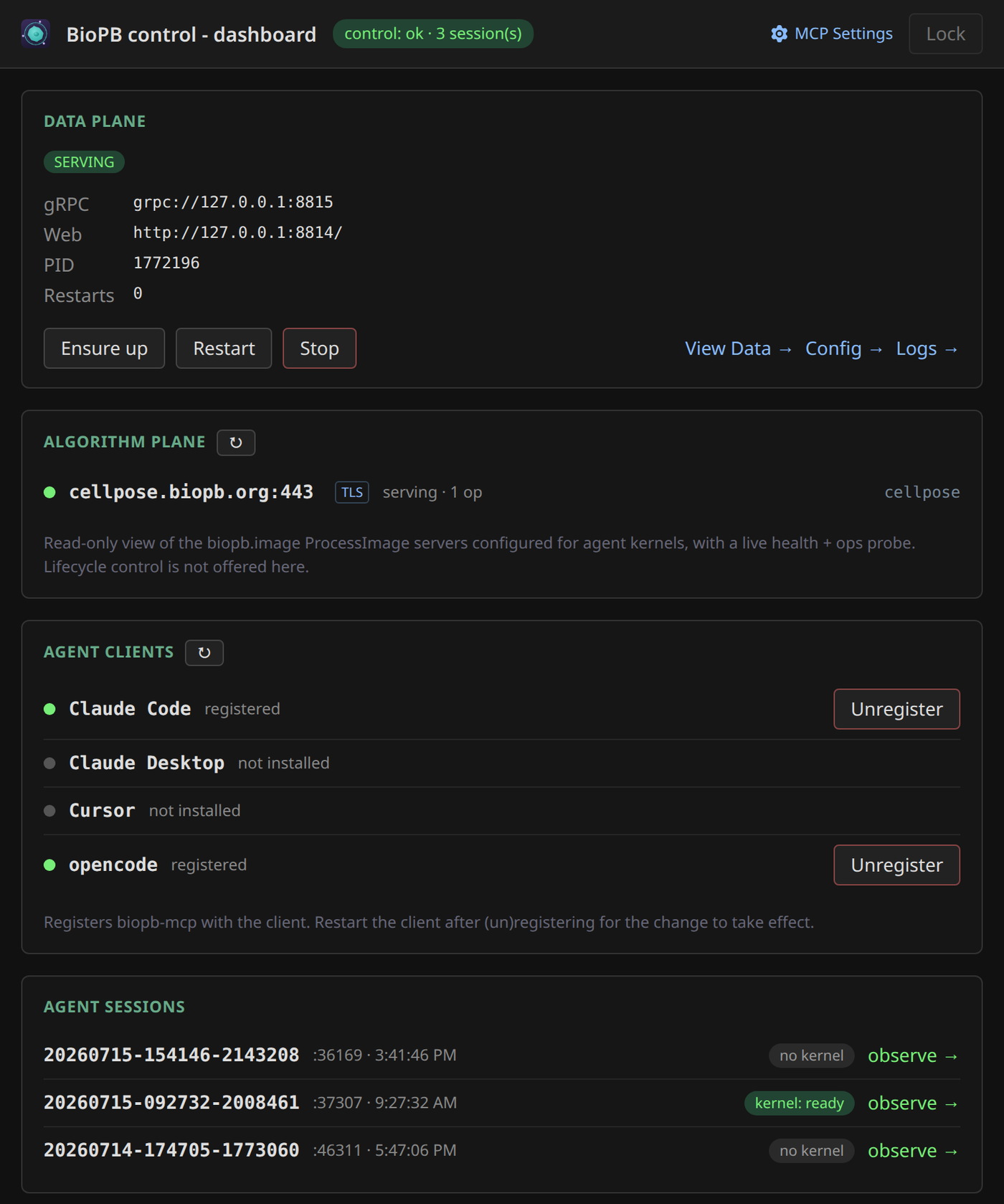
• Data plane — your data server's health and the buttons that drive it. Ensure up starts it if it isn't running (harmless if it already is), Restart bounces it, and Stop leaves clients without data until something asks for it again. Logs → opens its output, so you don't have to go digging through files.
• Algorithm plane — the algorithm servers your agent can reach, with a live health probe. Read-only: algorithm servers are started and stopped where they run, usually a GPU box or a container, not from here.
• Agent clients — register or unregister biopb with each agent; the same job as biopb agents register. Agents you don't have are listed as not installed and left alone. Restart the client afterwards, or it won't pick up the change.
• Agent sessions — every live session, its kernel state, and an observe → link. Each session is one agent's own viewer and kernel, so two agents means two rows here, not one shared session.

Watching your agent

An agent is a powerful but opaque collaborator. It writes and runs real Python on your machine — segmentations, measurements, file reads — and most of the time you only see the results, not the work. The observe view closes that gap. It exists so you can:

• See what's actually running. Every execute_code job shows up with its source and its captured output, newest first — so "what did the agent just do?" is always one glance away.
• Step in. If a job hangs or heads in the wrong direction, you can interrupt that one job or hard-restart the whole kernel — without killing the conversation.
• Keep a record. One click exports the entire session as a Jupyter notebook: an audit trail of every command the agent ran and what came back (see Saving a notebook (audit) below).

This is the same idea as the shared canvas in napari — you and the agent work over one session — applied to the code the agent runs rather than the images it produces.

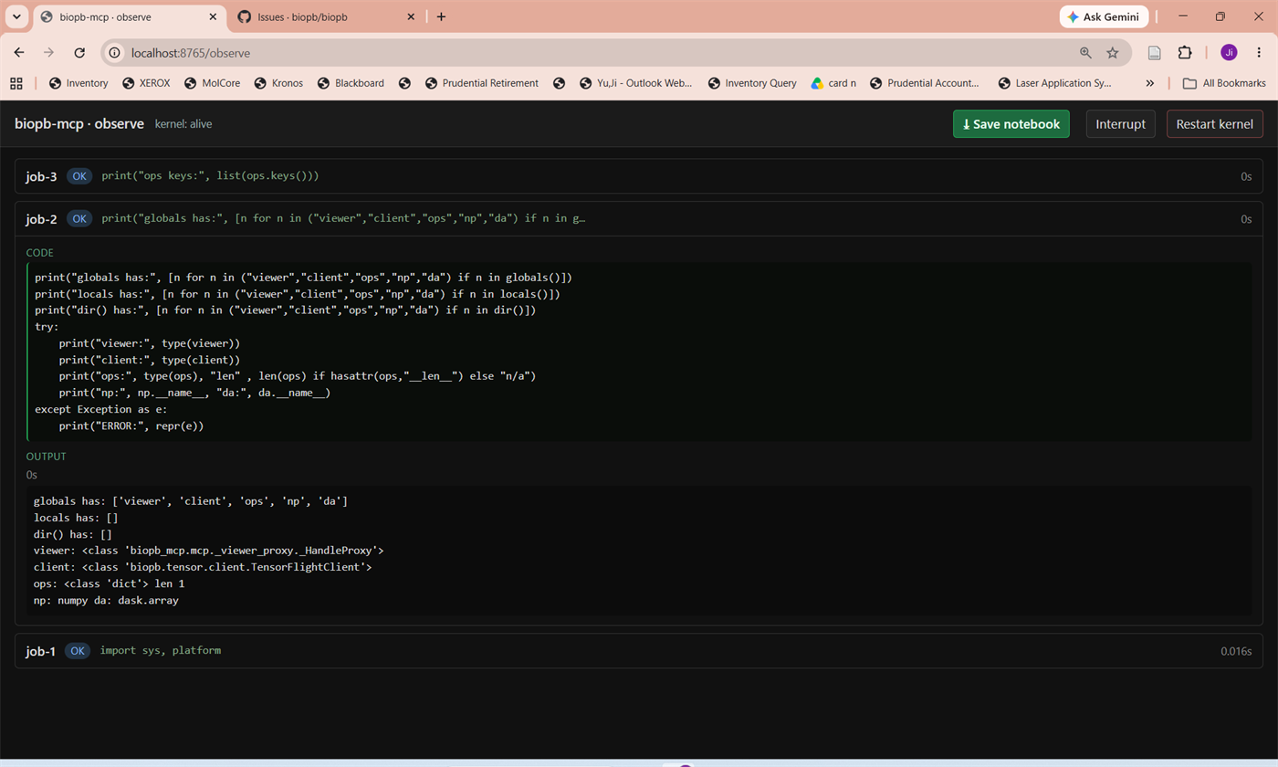
The observe view: recent execute_code jobs, newest first, with the kernel status and controls in the header.

Opening a session's view

Each agent session gets its own observe view. Open the dashboard and click the session you want under Agent sessions; that takes you to /session/<session-id>/observe.

There's no fixed URL to bookmark: every session runs on its own dynamically assigned port, and the control plane is what knows where each one lives. Going through the dashboard is how you find them. You can also ask your agent to run server_status, which reports the observe URL for its own session.

Reading the job list

Each row is one job the agent ran, with a status badge:

Badge	Meaning
running	The job is executing right now.
ok	Finished successfully.
error	Raised an exception (the traceback is in the output).
cancelled	Stopped by the agent.
interrupted	Stopped by you from this page.

Click a row to expand it and see the code that was run and its output. The newest job stays expanded automatically; older jobs collapse so the page doesn't get noisy. For a running job the output tails live as it's produced (long output is truncated to the most recent chunk, with the full length noted). The header shows the kernel state — alive, busy, headless — and refreshes every few seconds.

Stepping in

Three controls live in the header:

• Interrupt — forces a KeyboardInterrupt into the currently running job. Use this when a single command is stuck (a runaway loop, a stall) but the session is otherwise fine. The agent sees, through its normal result, that a user stopped the job — so it won't mistake the interruption for its own logic failing.
• Restart kernel — hard-restarts the Python kernel. This clears all variables and napari layers, so you're asked to confirm first. Reach for it when the kernel is wedged badly enough that interrupting one job isn't enough.
• ⤓ Save notebook — exports the session (covered next).

Interrupt the job, not the conversation

Interrupting or restarting from this page doesn't end your chat with the agent. The agent simply gets back a "stopped by user" result and you can tell it what to do next.

Saving a notebook (audit)

The ⤓ Save notebook button exports the whole recorded session as a standard Jupyter .ipynb file (biopb-mcp-session-YYYYMMDD-HHMMSS.ipynb). This is the view's most important feature for reproducibility and review.

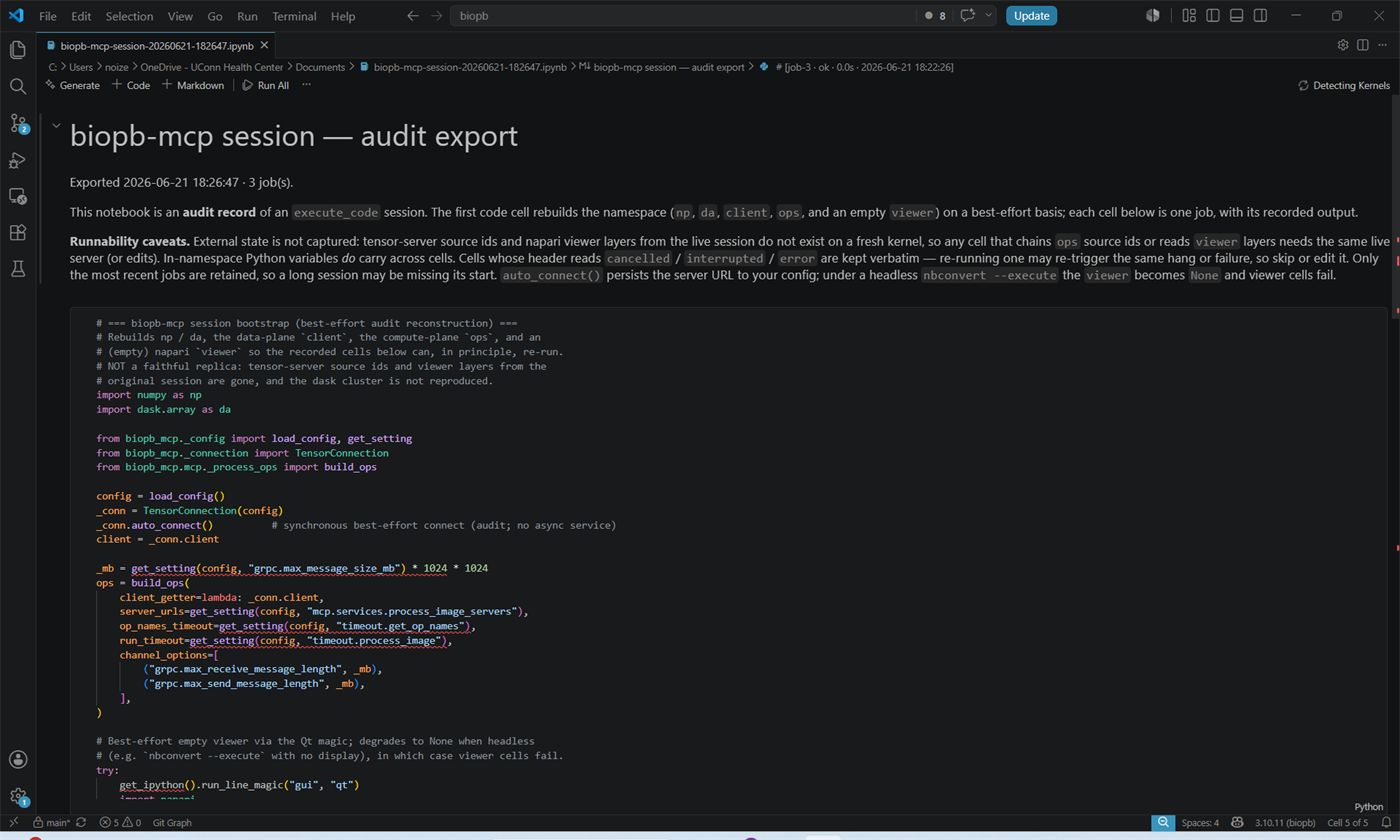
The notebook is an audit record first, a runnable script second. It faithfully reproduces, in order:

• a title and summary cell (when it was exported, how many jobs),
• a bootstrap cell that rebuilds the core namespace (np, da, the data-plane client, the compute-plane ops, and an empty napari viewer) on a best-effort basis, and
• one cell per job — the exact code the agent ran, with its captured stdout, results, and any error or interruption message — each headed by its job id, status, elapsed time, and timestamp.

That gives you a complete, shareable trail of what was done to your data: drop it next to your results, attach it to a paper's supplement, or hand it to a colleague to review.

The exported notebook: each cell is one job the agent ran, kept verbatim with its output and a header line.

Re-running has caveats

The notebook is meant to document a session, not perfectly replay it. In-namespace Python variables carry across cells, but external state is not captured: tensor-server source ids and the live napari layers from the original session may not coincide on a fresh kernel, so cells that chain ops source ids or read viewer layers need the same live server (or hand edits) to run again. Cells marked error, cancelled, or interrupted are kept verbatim — re-running one may re-trigger the same failure, so skip or edit it. Only the most recent jobs are retained, so a very long session may be missing its earliest steps.

Changing biopb settings

biopb keeps two config files, and the dashboard gives each one an editor so you don't have to hand-edit JSON:

• Config →, on the data plane panel, edits the data server's settings — where your data lives, the cache, the ports. This is biopb.json.
• MCP Settings, at the top right, edits biopb-mcp's settings — the kernel, dask, and the algorithm servers your agent can reach. This is mcp-config.json.

Both work the same way: change a value, then Save. The page tells you when you have unsaved changes, and refuses a value it can't accept rather than writing a broken file.

The data server reads its config at startup, so changes there take effect on the next Restart — the editor offers one, and the data plane panel has the same button. Editing settings won't silently restart anything under your agent.

The same values, either way

These editors and the config files are two doors onto the same settings. If you'd rather edit the files directly, Configuration documents the keys and where the files live.

Viewing your data

View Data →, on the data plane panel, opens biopb's web viewer. It lists the sources your data server is serving and lets you open and page through them in the browser.

It's the quickest way to check that your data is where you think it is, and what's actually in it — no agent, no napari, no waiting for a kernel to boot. The server renders the slice you're looking at and sends back just that picture, so even a dataset far larger than your machine opens immediately and your browser never downloads the pixels.

For real work — layers, editing, plugins, and a canvas you share with your agent — use napari instead.